On the wood price time series analysis:
A comparison between statistical and machine learning methods
By Dimitrios Koulialias and S. Swayamjyoti
Introduction
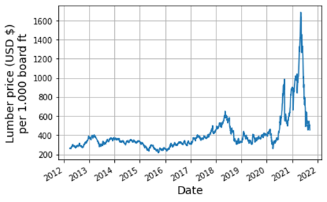
Since ancient times, wood has always been a significant resource to humankind, considering its manifold use for energy supply, paper production, or for construction purposes, to name a few examples. Despite its frequent usage to date, the economic value of wood to the global market is far less compared to other classic commodities such as gold or crude oil. Last year, however, this paradigm has changed drastically, given the fact that the wood / lumber price has undergone a striking increase from end of 2020, reaching an all-time high around 1600 US Dollars per 1000 board ft as of May 2021 (see Fig. 1)! It can be speculated that such increase in price has resulted from the aftereffects of the Covid-19 pandemic to the global economy, thus giving rise to an increasing imbalance between supply and demand. Given this and considering other long-term global factors that are susceptible to the wood supply, e.g., deforestation, wildfire, etc., it cannot be ruled out that its price evolution might become even more volatile in the future.
In this article, we are going to implement time series forecasting based on statistical and machine learning (ML) approaches using the lumber price evolution between 2012 and 2021 as a test bed. The closing price time series has been downloaded from [1]. For both approaches, a ratio of 90 : 10 was used for the splitting between the training and the test dataset. The implementation of the statistical and ML models was accomplished in Python.
1. Statistical time-series forecasting: the ARIMA model
1.1 General considerations
There have been several models proposed in the literature for time series analysis (e.g., see [2]). One popular and widely used among them is the ARIMA model, which is an acronym for Autoregressive Integrated Moving Average. It allows to make predictions on a time series based on its past values, i.e., the lags, as well as on its lagged forecast errors. The three components of the ARIMA model and their corresponding parameters (\( p,d,q \)) are defined as follows:
- AR(\(p\)) Autoregression: It indicates an autoregressive model of order \(p\) which states that the output variable \(y_t\) at time \(t\) is a linear combination of the previous \(t-p\) time lags \(y_{t-1}\), \(y_{t-2}\), …, \(y_{t-p}\), given by \begin{equation*} y_{t} = \alpha + \sum_{i=1}^p \beta_i y_{t-i} + \epsilon_t \end{equation*} where \(\beta_i \) are the regression parameters, \( \alpha \) is a constant, and \( \epsilon_t \) corresponds to the noise term.
- I(\(d\)) Integration: The integration parameter stands for the degree of differencing of observations, i.e., the subtraction of an observation from an observation of a previous time step for \(d\) number of times. The differentiation is of particular importance when it comes to transforming non-stationary data into a stationary one, which will be discussed further below.
- MA(\(q\)) Moving Average: This model establishes a relation between the output variable yt at time \(t\) and the previous \(q\) lagged errors of the time series as \begin{equation*} y_{t} = \alpha + \sum_{j=1}^q \gamma_j \epsilon_{t-j} + \epsilon_t \end{equation*} where the fitting parameters are defined in analogy to those of the autoregressive model.
Considering the above components, it becomes evident that the ARIMA model can be regarded as an extended regression model. In the following, the implementation of the ARIMA model to our lumber price time series is conducted.
1.2 Implementation of the ARIMA model
A general prerequisite for building any forecast model requires the data to be stationary, i.e., to have a nearly constant mean and variance / standard deviation over time. To test the stationarity of our lumber price evolution, we make use of the Augmented Dickey Fuller (ADF) test, which is a standardized approach for assessing the (non)-stationarity for a given time series (see e.g., [3]). This test relies on the null hypothesis, which states that the time series has a unit root, i.e., it is considered as non-stationary. A crucial quantity of the ADF test is the \(p\)-value, where for \(p\) < 0.05, there is a strong evidence against the null hypothesis, i.e., the time series can be considered as stationary, whereas for values greater than or equal to this threshold, it is considered as non-stationary, respectively. The ADF Test on our lumber price data yields \(p\) = 0.02. Therefore, we can state that our data in the given time range is stationary and this should be further reflected by obtaining a \(d = 0\) value when applying the ARIMA model below.
Based on the pmdarima package in Python, we apply the ‘auto_arima’ function to determine those parameters (\(p,d,q\)) that yield the best description with respect to the training dataset. The implementation yields the ARIMA(5, 0, 4) model as best approximation, i.e., an autoregression model with order five, a moving average model of order four, and an integration with order zero as expected. By fitting this model to the training set and applying that for making predictions with respect to the test set, we get the following forecast for the price evolution within a confidence interval of 95 % (Fig. 2)
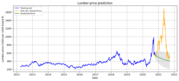
Apparently, it seems that the model evolves in a decreasing trend and covers only a little part of the actual price within the confidence interval. In the following, we will assess whether a better prediction can be achieved using the ML approach.
2. Time-series forecasting with Machine Learning
2.1 General considerations
The emergence of ML techniques in the last years and the rapidly evolving field in the development of
new kinds of neural networks (NN) has also prompted the use of ML for time series forecasting.
ML is a humongous field and rather than going in too much detail about it here, we would like to
briefly point out its key aspects (for a more detailed review about ML in general consider e.g., see [4]).
As a branch of artificial intelligence (AI), ML deals with the development of NN’s that aim to determine
complex relationships between large amounts of data (where “data” in this sense can be of any kind, e.g.,
numbers, text, images, classifications, etc.). Basically, a NN is a series of interconnected layers of
neurons with one input and one output layer across its ends (Fig. 3), and its functionality can be viewed
to be inspired by the biological neural networks that constitute the human brain. Assume that there are
two datasets, X and y\(_{act}\), whose relation is yet unknown. By giving X as input to the NN, it is transmitted
across the layers by undergoing certain mathematical operations until it reaches the output layer with a
predicted quantity y\(_{calc}\). This process is generally termed as feedforward. Compared with y\(_{act}\), i.e., the
actual quantity to be predicted, the resulting error
| y\(_{calc}\) - y\(_{act}\) | is calculated and propagated back
to the NN, and the transmission weights between the neuron layers are modified in such a way that this
error becomes minimal; hence this reverse process is called backpropagation. Given this, the NN can be
trained to predict the desired output by accomplishing a series of feedforward and backpropagation
processes on the training dataset (X\(_{train}\), y\(_{train}\)). The number of one full feedforward and backpropagation
cycle over the entire training dataset is called an epoch. Once trained, the NN is applied to the
remaining test dataset (X\(_{test}\), y\(_{test}\)) and depending on how good the accuracy is, the NN can either be
used for predictions, or it needs further improvement through additional training.
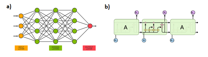
Considering the NN schema as illustrated in Figure 3a, it refers to one of the simplest and one of the very first developed NN architectures, which is the multi-layer perceptron (MLP). Nowadays, depending on the complexity of the underlying problem, there are many other architectures available for use, and they are designed in such a way that they fit specialized tasks better than an MLP would.
A more complex NN that is commonly used on temporal sequence datasets is the recurrent neural network (RNN) that refers to a class of NN architectures, in which connections between nodes form a directed graph along a temporal sequence. For our problem, we make the use of an LSTM (Long Short-Term Memory) network, which is a special kind of RNN. In particular, an LSTM memory cell as depicted in Fig. 3b) has a more elaborate internal architecture that allows to store and retrieve relevant information over a long-term sequence. Further details on the RNN and LSTM architectures can be found in [6].
2.2 Implementation of the LSTM model
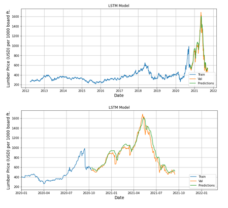
The model architecture has been built up by a sequence of two LSTM layers and two dense layers. Considering that the number of lags is equal to five trading days as inferred from the ARIMA model, we used this value to define the number of LSTM nodes. For the first dense layer, we chose four nodes, and for the last one, only a single node has been assigned, given that we expect a single output. With this in mind, the training of the model has been accomplished with a batch size equal to one and one single epoch.
By applying the trained model to the test dataset, the accuracy as defined in terms of the root mean squared error (RMSE) amounts to 40.8. This value is pretty decent, given that the range of the time series is at least one order of magnitude higher. Overall, this results in a relatively concise description of the between the actual and the calculated test datasets (Fig. 4).
Summary
In this article, we used the lumber price in order to estimate its evolution based on statistical and ML predictive time-series approaches. The former approach using the ARIMA model provided an inadequate description of the test set. In contrast, the ML approach performed much better and was able to describe the peak anomaly that was attained during spring 2021.
Given that we used the closing price as the only parameter and considering the above outcome, our findings shall not be interpreted in a way that they favor one approach over the other. Instead, they should be regarded as an educational example to demonstrate the use of predictive time-series approaches on the manifold universe of asset classes.